期权波动率交易策略:从Vega到实战#
引言:波动率是期权交易的核心#
在股票市场中,我们交易的是价格;在期权市场中,我们交易的是波动率。
期权的价格不仅取决于标的资产的现价,更取决于市场对未来波动率的预期。这就是为什么专业期权交易员说:
“方向不重要,波动率才重要。”
本文将深入探讨:
- 波动率的基本概念与度量
- 期权希腊字母中的Vega
- 波动率曲面(Volatility Surface)
- 实盘波动率交易策略
一、波动率:从概念到度量#
1.1 什么是波动率?#
波动率(Volatility)衡量的是资产价格变动的剧烈程度,通常用年化标准差表示。
两种波动率:
- 历史波动率(Historical Volatility):基于过去价格计算的实际波动率
- 隐含波动率(Implied Volatility, IV):从期权价格反推的市场预期波动率
1.2 历史波动率计算#
import numpy as np
import pandas as pd

def calculate_historical_volatility(price_series, window=20, annualize=True):
    """
    计算历史波动率

    Parameters:
    -----------
    price_series : Series
        价格序列(如收盘价)
    window : int
        滚动窗口大小(交易日)
    annualize : bool
        是否年化(乘以√252)

    Returns:
    --------
    hv : Series
        历史波动率序列
    """
    # 计算对数收益率
    log_returns = np.log(price_series / price_series.shift(1))

    # 滚动标准差
    hv = log_returns.rolling(window=window).std()

    # 年化
    if annualize:
        hv = hv * np.sqrt(252)

    return hv * 100  # 转换为百分比

# 使用示例
# hv = calculate_historical_volatility(stock_data['close'], window=20)1.3 隐含波动率计算#
隐含波动率是通过B-S公式反推得到的。给定期权价格,求解使得B-S公式成立的波动率参数。
from scipy.optimize import brentq
from scipy.stats import norm

def black_scholes_price(S, K, T, r, sigma, option_type='call'):
    """
    Black-Scholes期权定价公式

    Parameters:
    -----------
    S : float
        标的资产现价
    K : float
        行权价
    T : float
        剩余期限(年)
    r : float
        无风险利率
    sigma : float
        波动率
    option_type : str
        'call' 或 'put'

    Returns:
    --------
    price : float
        期权理论价格
    """
    d1 = (np.log(S / K) + (r + 0.5 * sigma**2) * T) / (sigma * np.sqrt(T))
    d2 = d1 - sigma * np.sqrt(T)

    if option_type == 'call':
        price = S * norm.cdf(d1) - K * np.exp(-r * T) * norm.cdf(d2)
    elif option_type == 'put':
        price = K * np.exp(-r * T) * norm.cdf(-d2) - S * norm.cdf(-d1)

    return price

def implied_volatility(market_price, S, K, T, r, option_type='call',
                       sigma_min=0.01, sigma_max=5.0):
    """
    计算隐含波动率(使用Brent方法求解)

    Parameters:
    -----------
    market_price : float
        期权市场价格
    S, K, T, r : float
        同上
    option_type : str
        'call' 或 'put'
    sigma_min, sigma_max : float
        波动率搜索区间

    Returns:
    --------
    iv : float
        隐含波动率
    """
    def objective(sigma):
        return black_scholes_price(S, K, T, r, sigma, option_type) - market_price

    try:
        iv = brentq(objective, sigma_min, sigma_max, xtol=1e-6)
        return iv * 100  # 转换为百分比
    except ValueError:
        return np.nan

# 使用示例
# market_price = 5.20  # 期权市场价格
# iv = implied_volatility(market_price, S=100, K=100, T=0.25, r=0.03, option_type='call')
# print(f"隐含波动率: {iv:.2f}%")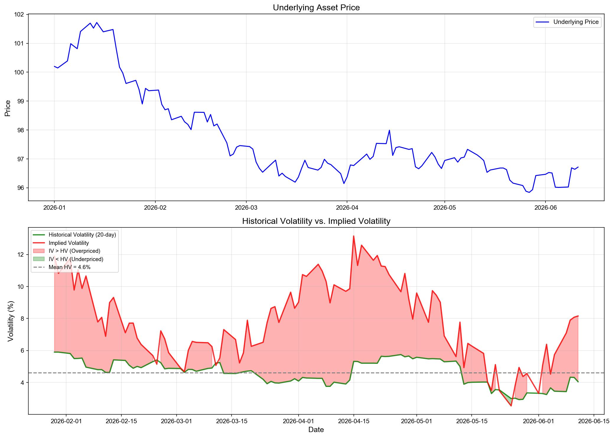
二、Vega:波动率敏感度#
2.1 希腊字母回顾#
期权的价格受多个因素影响,希腊字母(Greeks)衡量的是期权价格对这些因素的敏感度:
| 希腊字母 | 定义 | 物理意义 |
|---|---|---|
| Delta (Δ) | ∂C/∂S | 标的资产价格变动1元,期权价格变动多少 |
| Gamma (Γ) | ∂²C/∂S² | Delta的变化率 |
| Theta (Θ) | ∂C/∂t | 时间衰减 |
| Vega (ν) | ∂C/∂σ | 波动率变动1%,期权价格变动多少 |
| Rho (ρ) | ∂C/∂r | 无风险利率变动的影响 |
2.2 Vega的计算与特征#
Vega公式(B-S模型):
Vega = S * √(T) * N'(d1)其中 N’(d1) 是标准正态概率密度函数。
Vega的特征:
- 正值:无论看涨还是看跌期权,Vega通常为正(波动率上升→期权价格上升)
- 期限结构:长期期权的Vega大于短期期权
- 行权价结构:平值期权(ATM)的Vega最大
def calculate_vega(S, K, T, r, sigma):
    """
    计算Vega

    Parameters:
    -----------
    S, K, T, r, sigma : float
        同black_scholes_price

    Returns:
    --------
    vega : float
        Vega值(每1%波动率变动,期权价格变动多少)
    """
    d1 = (np.log(S / K) + (r + 0.5 * sigma**2) * T) / (sigma * np.sqrt(T))

    # 标准正态概率密度函数
    n_prime_d1 = norm.pdf(d1)

    # Vega (除以100,因为波动率通常以百分比表示)
    vega = S * np.sqrt(T) * n_prime_d1 / 100

    return vega

# Vega随行权价变化示例
strikes = np.linspace(80, 120, 41)
vegas = [calculate_vega(S=100, K=K, T=0.25, r=0.03, sigma=0.25) for K in strikes]

import matplotlib.pyplot as plt
plt.figure(figsize=(10, 6))
plt.plot(strikes, vegas, 'b-', linewidth=2)
plt.axvline(x=100, color='r', linestyle='--', label='ATM (K=100)')
plt.xlabel('Strike Price')
plt.ylabel('Vega')
plt.title('Vega vs. Strike Price (T=0.25, σ=25%)')
plt.legend()
plt.grid(True)
plt.show()2.3 Vega在交易中的应用#
场景一:做多波动率(Long Volatility)
- 策略:买入跨式组合(Long Straddle)——同时买入看涨和看跌期权
- 盈亏:获利当实际波动率 > 隐含波动率
- 风险:时间衰减(Theta为负)
场景二:做空波动率(Short Volatility)
- 策略:卖出跨式组合(Short Straddle)
- 盈亏:获利当实际波动率 < 隐含波动率
- 风险:无限亏损风险(需严格止损)
三、波动率曲面:从微笑到倾斜#
3.1 波动率微笑(Volatility Smile)#
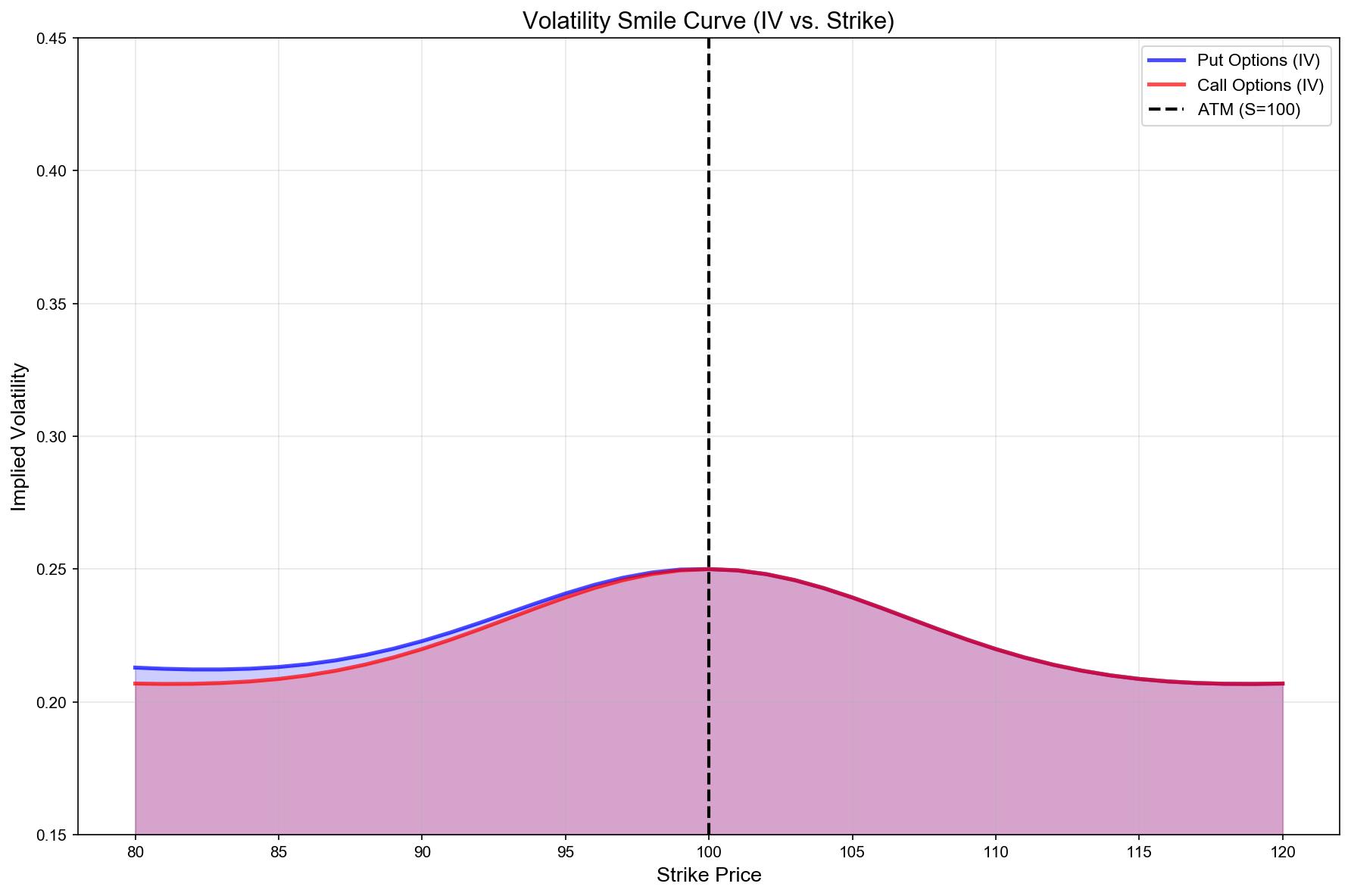
观察: 相同到期日、不同行权价的期权,其隐含波动率并不相同,而是呈现微笑曲线(Smile)或倾斜曲线(Skew)。
原因:
- 杠杆效应:下跌时波动率往往上升(恐慌情绪)
- 供需失衡:看跌期权的需求更大(对冲需求)
- 跳跃风险:市场崩盘时,虚值看跌期权价值飙升
3.2 构建波动率曲面#
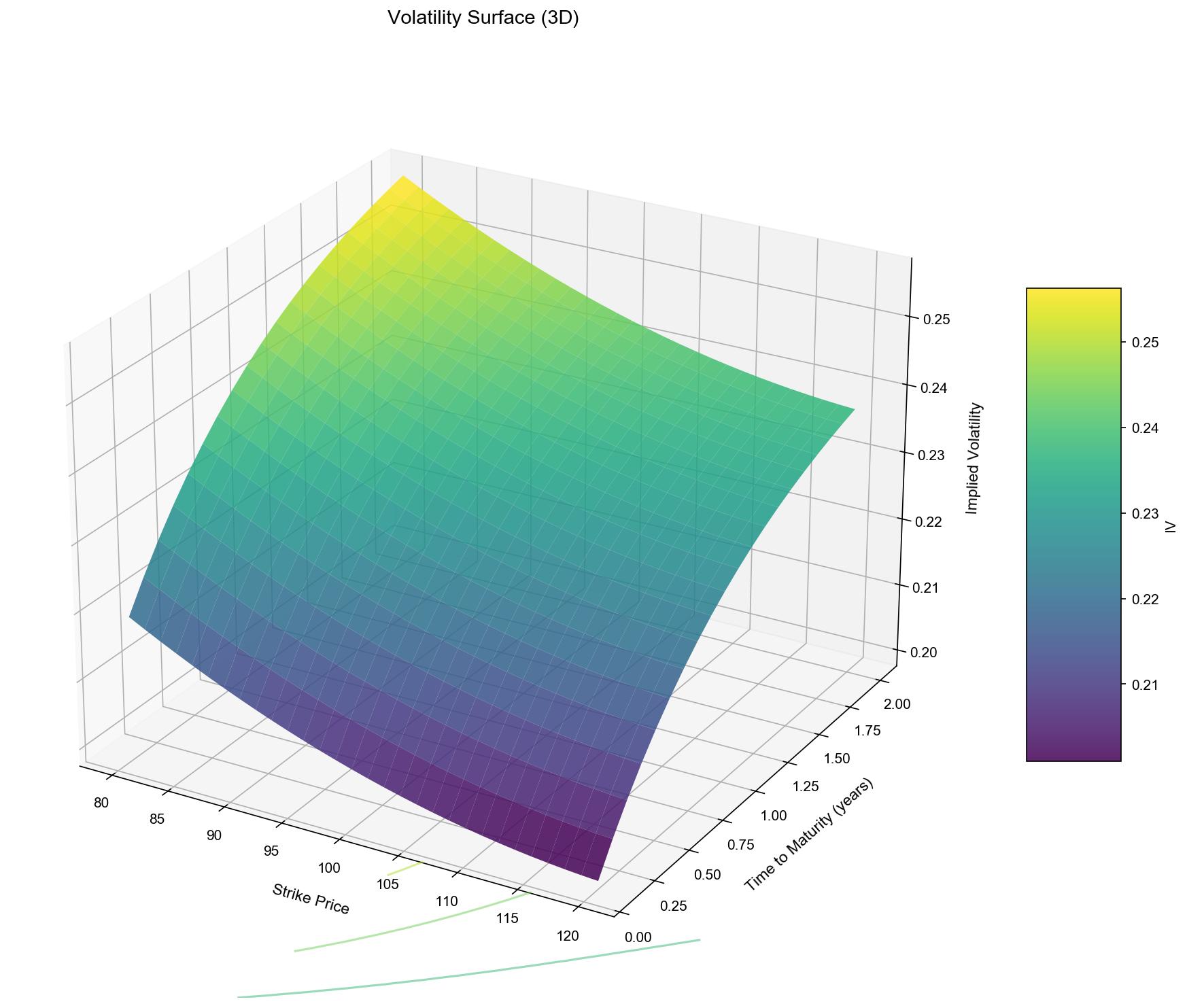
波动率曲面(Volatility Surface)是期限结构(不同到期日)和微笑曲线(不同行权价)的二维展示。
def build_volatility_surface(options_data):
    """
    构建波动率曲面

    Parameters:
    -----------
    options_data : DataFrame
        包含columns: ['strike', 'maturity', 'implied_vol']
        - strike: 行权价
        - maturity: 剩余期限(年)
        - implied_vol: 隐含波动率(%)

    Returns:
    --------
    vol_surface : Axes3D
        波动率曲面图
    """
    from mpl_toolkits.mplot3d import Axes3D

    # 准备数据
    K = options_data['strike'].values
    T = options_data['maturity'].values
    IV = options_data['implied_vol'].values / 100  # 转换为小数

    # 插值(使用cubic spline)
    from scipy.interpolate import griddata

    # 创建网格
    K_grid = np.linspace(K.min(), K.max(), 50)
    T_grid = np.linspace(T.min(), T.max(), 50)
    K_mesh, T_mesh = np.meshgrid(K_grid, T_grid)

    # 插值
    IV_mesh = griddata((K, T), IV, (K_mesh, T_mesh), method='cubic')

    # 绘图
    fig = plt.figure(figsize=(12, 8))
    ax = fig.add_subplot(111, projection='3d')
    surf = ax.plot_surface(K_mesh, T_mesh, IV_mesh, cmap='viridis',
                           alpha=0.8, antialiased=True)

    ax.set_xlabel('Strike Price')
    ax.set_ylabel('Time to Maturity (years)')
    ax.set_zlabel('Implied Volatility')
    ax.set_title('Volatility Surface')
    fig.colorbar(surf, shrink=0.5, aspect=5)
    plt.show()

    return fig

# 使用示例(需要真实数据)
# vol_surface = build_volatility_surface(options_data)3.3 波动率套利(Volatility Arbitrage)#
策略逻辑: 当不同期权合约的隐含波动率出现异常偏离时,可以通过买入低估期权、卖出高估期权来获取无风险利润。
常见套利机会:
- 水平套利(Calendar Spread):同一行权价、不同到期日的IV差异
- 垂直套利(Vertical Spread):同一到期日、不同行权价的IV差异
- 对角套利(Diagonal Spread):行权价和到期日都不同
def detect_vol_arb_opportunity(options_chain, threshold=0.05):
    """
    检测波动率套利机会

    Parameters:
    -----------
    options_chain : DataFrame
        期权链数据,包含['strike', 'maturity', 'call_iv', 'put_iv', 'call_price', 'put_price']
    threshold : float
        IV差异阈值(5%)

    Returns:
    --------
    opportunities : list
        套利机会列表
    """
    opportunities = []

    # 1. 检测水平套利机会(同一strike,不同maturity)
    for strike in options_chain['strike'].unique():
        subset = options_chain[options_chain['strike'] == strike].sort_values('maturity')
        for i in range(len(subset) - 1):
            iv_diff = abs(subset.iloc[i]['call_iv'] - subset.iloc[i+1]['call_iv'])
            if iv_diff > threshold:
                opportunities.append({
                    'type': 'calendar_spread',
                    'strike': strike,
                    'maturity_1': subset.iloc[i]['maturity'],
                    'maturity_2': subset.iloc[i+1]['maturity'],
                    'iv_diff': iv_diff,
                    'trade': 'Buy low IV, Sell high IV'
                })

    # 2. 检测垂直套利机会(同一maturity,不同strike)
    for maturity in options_chain['maturity'].unique():
        subset = options_chain[options_chain['maturity'] == maturity].sort_values('strike')
        for i in range(len(subset) - 1):
            iv_diff = abs(subset.iloc[i]['call_iv'] - subset.iloc[i+1]['call_iv'])
            if iv_diff > threshold:
                opportunities.append({
                    'type': 'vertical_spread',
                    'maturity': maturity,
                    'strike_1': subset.iloc[i]['strike'],
                    'strike_2': subset.iloc[i+1]['strike'],
                    'iv_diff': iv_diff,
                    'trade': 'Buy low IV, Sell high IV'
                })

    return opportunities

# 使用示例
# opportunities = detect_vol_arb_opportunity(options_chain, threshold=0.05)
# for opp in opportunities:
# print(opp)四、实盘波动率交易策略#
4.1 策略一:Delta对冲的波动率交易#
核心思想: 通过动态对冲Delta,将期权头寸转化为纯波动率头寸。
步骤:
- 买入期权(做多波动率)
- 动态卖出/买入标的资产,使整体Delta接近0
- 获利来源:实际波动率 > 隐含波动率
class DeltaHedgedVolTrade:
    def __init__(self, option_position, underlying, initial_delta):
        self.option_position = option_position  # 期权持仓(正数=多头)
        self.underlying = underlying  # 标的资产代码
        self.delta = initial_delta  # 当前Delta
        self.hedge_position = 0  # 对冲持仓(负数=卖出)

    def rebalance_hedge(self, new_delta):
        """重新平衡对冲头寸"""
        # 计算需要交易的标的资产数量
        trade_size = - (new_delta * self.option_position + self.hedge_position)

        # 执行交易(简化版,假设无交易成本)
        self.hedge_position += trade_size

        print(f"Rebalance: Trade {trade_size:.0f} shares of {self.underlying}")
        print(f"New hedge position: {self.hedge_position:.0f}")

        self.delta = new_delta

    def calculate_pnl(self, option_pnl, underlying_pnl):
        """计算总盈亏"""
        total_pnl = option_pnl + underlying_pnl * self.hedge_position
        return total_pnl

# 使用示例
# trade = DeltaHedgedVolTrade(option_position=10, underlying='510050.SH', initial_delta=0.5)
# trade.rebalance_hedge(new_delta=0.6) # Delta从0.5变为0.6,需要卖出更多标的4.2 策略二:跨式组合(Straddle)交易#
策略逻辑: 同时买入相同行权价、相同到期日的看涨和看跌期权,从大幅波动中获利(无论方向)。
适用场景:
- 重大事件前夕(财报、FOMC会议、选举)
- 隐含波动率较低时
- 预期市场将出现剧烈波动
def backtest_straddle_strategy(underlying_data, options_data, event_dates,
                                entry_days_before=5, exit_days_after=1):
    """
    回测跨式组合策略

    Parameters:
    -----------
    underlying_data : DataFrame
        标的资产数据,包含['date', 'close']
    options_data : DataFrame
        期权数据,包含['date', 'strike', 'maturity', 'call_price', 'put_price', 'iv']
    event_dates : list
        重大事件日期(如财报日)
    entry_days_before : int
        事件前多少天入场
    exit_days_after : int
        事件后多少天出场

    Returns:
    --------
    results : DataFrame
        回测结果
    """
    results = []

    for event_date in event_dates:
        # 入场日期
        entry_date = event_date - pd.Timedelta(days=entry_days_before)
        # 出场日期
        exit_date = event_date + pd.Timedelta(days=exit_days_after)

        # 找到最接近的期权(平值、近月)
        entry_options = options_data[options_data['date'] == entry_date]
        atm_option = entry_options.iloc[abs(entry_options['strike'] -
                                            underlying_data.loc[entry_date, 'close']).idxmin()]

        # 计算成本
        entry_cost = atm_option['call_price'] + atm_option['put_price']

        # 出场时的期权价值
        exit_options = options_data[options_data['date'] == exit_date]
        exit_option_call = exit_options[exit_options['strike'] == atm_option['strike']].iloc[0]['call_price']
        exit_option_put = exit_options[exit_options['strike'] == atm_option['strike']].iloc[0]['put_price']
        exit_value = exit_option_call + exit_option_put

        # 盈亏
        pnl = exit_value - entry_cost
        pnl_pct = pnl / entry_cost * 100

        results.append({
            'event_date': event_date,
            'entry_date': entry_date,
            'exit_date': exit_date,
            'entry_iv': atm_option['iv'],
            'underlying_move': (underlying_data.loc[exit_date, 'close'] -
                               underlying_data.loc[entry_date, 'close']) /
                               underlying_data.loc[entry_date, 'close'] * 100,
            'pnl': pnl,
            'pnl_pct': pnl_pct
        })

    return pd.DataFrame(results)

# 使用示例
# results = backtest_straddle_strategy(stock_data, options_chain, event_dates,
#                                       entry_days_before=5, exit_days_after=1)
# print(results[['event_date', 'entry_iv', 'underlying_move', 'pnl_pct']])4.3 策略三:波动率风险溢价(VRP)策略#
策略逻辑: 隐含波动率(IV)通常高于实际波动率(RV),这个差额称为波动率风险溢价(Volatility Risk Premium, VRP)。我们可以通过卖出期权来赚取这个溢价。
VRP计算公式:
VRP = IV - RV交易规则:
- 当 VRP > 阈值(如5%)时,卖出跨式组合(Short Straddle)
- 当 VRP < 阈值时,平仓或反向操作
def compute_vrp(options_data, underlying_returns, window=20):
    """
    计算波动率风险溢价(VRP)

    Parameters:
    -----------
    options_data : DataFrame
        期权数据,包含['date', 'iv'](平均IV)
    underlying_returns : Series
        标的资产收益率
    window : int
        计算实际波动率的窗口

    Returns:
    --------
    vrp : DataFrame
        VRP序列
    """
    # 计算实际波动率(RV)
    rv = underlying_returns.rolling(window=window).std() * np.sqrt(252) * 100

    # 合并数据
    data = pd.DataFrame({
        'date': options_data['date'],
        'iv': options_data['iv']
    }).set_index('date')
    data['rv'] = rv

    # 计算VRP
    data['vrp'] = data['iv'] - data['rv']

    return data[['iv', 'rv', 'vrp']]

def trade_vrp_strategy(vrp_data, threshold=5.0):
    """
    VRP交易策略

    Parameters:
    -----------
    vrp_data : DataFrame
        包含['iv', 'rv', 'vrp']
    threshold : float
        VRP阈值(%)

    Returns:
    --------
    signals : Series
        交易信号(1=做空波动率,0=平仓,-1=做多波动率)
    """
    signals = pd.Series(index=vrp_data.index, data=0)

    signals[vrp_data['vrp'] > threshold] = 1   # 卖出期权(做空波动率)
    signals[vrp_data['vrp'] < -threshold] = -1  # 买入期权(做多波动率)

    return signals

# 使用示例
# vrp_data = compute_vrp(options_chain, stock_returns, window=20)
# signals = trade_vrp_strategy(vrp_data, threshold=5.0)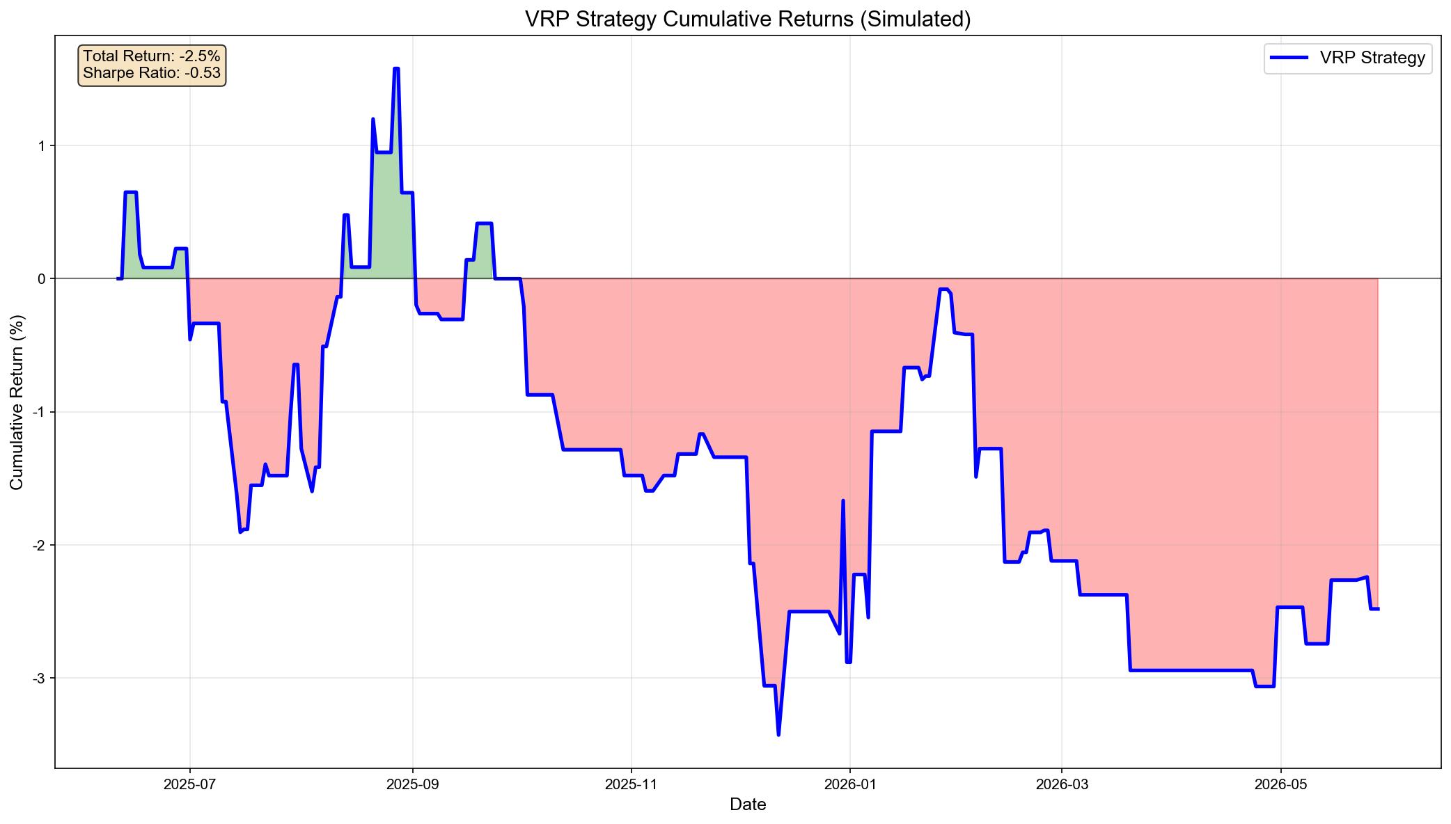
五、风险管理与实战建议#
5.1 期权交易的特殊风险#
| 风险类型 | 说明 | 应对方法 |
|---|---|---|
| Delta风险 | 标的资产价格变动 | 动态对冲 |
| Gamma风险 | Delta加速变化 | 限制头寸规模 |
| Theta风险 | 时间衰减 | 避免持有近月期权过长时间 |
| Vega风险 | 波动率突变 | 分散到期日和行权价 |
| 流动性风险 | 买卖价差过大 | 选择主力合约 |
5.2 仓位管理#
期权交易的高杠杆特性要求严格的仓位管理:
def kelly_criterion_option_trade(win_prob, win_amount, lose_amount):
    """
    使用凯利公式计算最优仓位

    Parameters:
    -----------
    win_prob : float
        胜率(0-1)
    win_amount : float
        获胜时的收益倍数
    lose_amount : float
        失败时的亏损倍数(正数)

    Returns:
    --------
    kelly_fraction : float
        凯利比例(建议实际使用半凯利或1/4凯利)
    """
    kelly = (win_prob * win_amount - (1 - win_prob) * lose_amount) / win_amount
    return max(0, min(kelly, 1))  # 限制在0-1之间

# 示例:跨式组合交易
# 胜率40%,获胜时收益200%,失败时亏损100%
kelly = kelly_criterion_option_trade(win_prob=0.4, win_amount=2.0, lose_amount=1.0)
print(f"凯利比例: {kelly:.2%}") # 建议实际使用 0.5*kelly 或 0.25*kelly5.3 实盘注意事项#
- 交易成本:期权买卖价差大,频繁交易会侵蚀利润
- 滑点:市场剧烈波动时,期权价格跳空
- 提前行权风险:美式期权可能被提前行权
- 保证金管理:卖出期权需要缴纳保证金,防止爆仓
六、总结与展望#
期权波动率交易是量化交易的**“高级领域”**,它要求:
- 数学功底:B-S公式、随机微积分、蒙特卡洛模拟
- 编程能力:期权定价、希腊字母计算、波动率曲面建模
- 市场理解:波动率期限结构、期限结构套利、事件驱动
未来趋势:
- AI在期权定价中的应用:神经网络逼近复杂期权价格
- 高频期权交易:利用订单流数据捕捉期权微观结构机会
- 结构化产品:将期权组合打包成自动化产品
免责声明: 本文仅供学习交流,不构成投资建议。期权交易风险极高,请在充分理解风险的前提下谨慎参与。
参考资料:
- Hull, J. C. (2022). Options, Futures, and Other Derivatives (11th Edition). Pearson.
- Gatheral, J. (2006). The Volatility Surface: A Practitioner’s Guide. Wiley.
- 上海证券交易所. (2023). 股票期权交易规则.