最优执行算法详解：从VWAP到强化学习驱动的现代交易系统 • halo 的技术博客

引言#

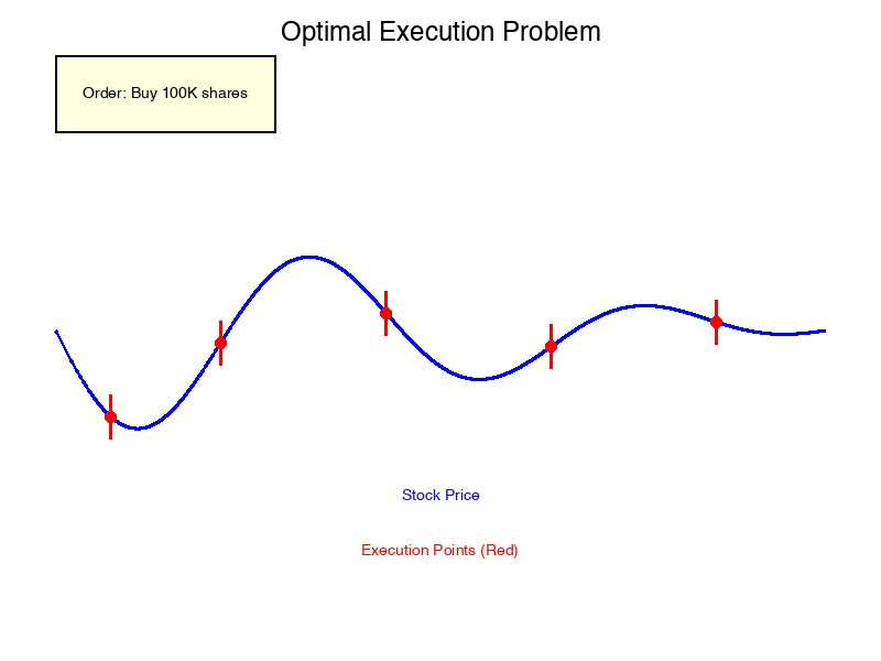
如果你有一个100万股的买入订单，你会如何执行？

一次性买入？ 市场冲击巨大，滑点可能吞噬全部收益。

慢慢买入？ 市场可能朝不利方向运行，机会成本太高。

这就是最优执行算法（Optimal Execution Algorithms）要解决的问题：在最小化市场冲击和最小化时间风险之间找到平衡，以最优价格完成订单。

在量化交易的世界里，策略生成阿尔法只是第一步，执行质量往往决定了最终的实盘收益。本文将深入剖析：

经典执行算法：VWAP、TWAP、POV、IS
现代方法：基于机器学习和强化学习的执行优化
实盘应用中的关键挑战（隐藏单、冰山单、暗池）
Python实战：构建一个VWAP执行引擎

执行问题的形式化定义#

1. 目标函数#

假设我们需要买入 $Q$ 股，时间窗口为 $[0, T]$ 。

定义：

$x(t)$ ：时刻 $t$ 的剩余数量
$v(t)$ ：时刻 $t$ 的执行速率（股/分钟）
$P(t)$ ：时刻 $t$ 的市场价格
$S(t)$ ：累计执行数量

目标：最小化总执行成本

\min_{v(t)} \int_0^T [P(t) + \lambda v(t)^\alpha] v(t) dt

其中：

第一项：支付的资金（价格 × 数量）
第二项：市场冲击成本（通常是非线性的， $α ≈ 0.5-1.5$ ）
$λ$ ：市场冲击系数

2. 约束条件#

完成约束： $\int_0^T v(t) dt = Q$
速率约束： $0 \leq v(t) \leq v_{max}$
参与度约束： $v(t) \leq γ \cdot V(t)$ （不超过市场成交量的 $γ$ ）

最优执行问题示意图

经典执行算法#

1. VWAP (Volume Weighted Average Price)#

核心思想：按照市场成交量的时间分布，等比例执行订单，使执行均价接近VWAP。

执行曲线：

v(t) = \frac{Q}{\int_0^T V(s) ds} \cdot V(t)

其中 $V(t)$ 是时刻 $t$ 的预测成交量。

Python实现：

import numpy as np
import pandas as pd

class VWAPExecution:
    def __init__(self, total_quantity, time_windows, volume_profile):
        """
        初始化VWAP执行器
        
        Parameters:
        -----------
        total_quantity : int
            总执行数量
        time_windows : array-like
            时间窗口（分钟）
        volume_profile : array-like
            每个时间窗口的预测成交量（股）
        """
        self.total_quantity = total_quantity
        self.time_windows = time_windows
        self.volume_profile = np.array(volume_profile)
        
        # 计算VWAP执行曲线
        self.execution_schedule = self._calculate_schedule()
    
    def _calculate_schedule(self):
        """计算VWAP执行计划"""
        total_volume = np.sum(self.volume_profile)
        
        # 每个时间窗口的执行数量 = 总数量 × (窗口成交量 / 总成交量)
        schedule = self.total_quantity * self.volume_profile / total_volume
        
        return schedule
    
    def execute(self, current_time, market_volume):
        """
        执行订单
        
        Parameters:
        -----------
        current_time : int
            当前时间窗口索引
        market_volume : float
            当前窗口的实际成交量
        
        Returns:
        --------
        execution_quantity : float
            本窗口应执行数量
        """
        # 按照计划执行
        planned_quantity = self.execution_schedule[current_time]
        
        # 限制：不超过市场成交量的一定比例（如20%）
        max_participation = 0.2 * market_volume
        execution_quantity = min(planned_quantity, max_participation)
        
        return execution_quantity
    
    def get_schedule_df(self):
        """返回执行计划DataFrame"""
        return pd.DataFrame({
            'time_window': self.time_windows,
            'planned_quantity': self.execution_schedule,
            'cumulative_quantity': np.cumsum(self.execution_schedule)
        })

# 使用示例
time_windows = np.arange(0, 390)  # 390分钟（6.5小时交易时间）
volume_profile = np.exp(-0.01 * time_windows) * 10000  # 模拟成交量衰减

vwap = VWAPExecution(total_quantity=100000, time_windows=time_windows, volume_profile=volume_profile)
schedule_df = vwap.get_schedule_df()
print(schedule_df.head())

python

优点：

简单易懂
跟踪基准明确（VWAP）
适合流动性好的大盘股

缺点：

被动跟随市场，无法利用价格预测
对市场冲击模型假设过于简化

2. TWAP (Time Weighted Average Price)#

核心思想：均匀分配执行数量到每个时间窗口。

执行曲线：

v(t) = \frac{Q}{T}

Python实现：

class TWAPExecution:
    def __init__(self, total_quantity, num_windows):
        self.total_quantity = total_quantity
        self.num_windows = num_windows
        self.quantity_per_window = total_quantity / num_windows
    
    def execute(self, current_window):
        """每个窗口执行相同数量"""
        return self.quantity_per_window

# 使用示例
twap = TWAPExecution(total_quantity=100000, num_windows=390)
print(f"每5分钟执行: {twap.quantity_per_window:.0f} 股")

python

优点：

极其简单
确定性执行计划

缺点：

忽略成交量分布（可能在高成交量时段执行不足）
容易被识别为算法交易（网络游戏）

3. POV (Percentage of Volume)#

核心思想：按照市场成交量的固定比例执行。

执行曲线：

v(t) = γ \cdot V(t)

其中 $γ$ 是参与度参数（如10%）。

动态调整：

class POVExecution:
    def __init__(self, total_quantity, target_participation=0.1, max_participation=0.2):
        self.total_quantity = total_quantity
        self.target_participation = target_participation
        self.max_participation = max_participation
        self.executed_quantity = 0
    
    def execute(self, market_volume):
        """根据市场成交量动态调整"""
        if self.executed_quantity >= self.total_quantity:
            return 0
        
        # 目标执行数量
        target_quantity = market_volume * self.target_participation
        
        # 剩余需要执行的数量
        remaining = self.total_quantity - self.executed_quantity
        
        # 实际执行数量（不超过剩余数量和市场限制）
        execution_quantity = min(target_quantity, remaining, market_volume * self.max_participation)
        
        self.executed_quantity += execution_quantity
        
        return execution_quantity

python

优点：

自动适应市场流动性
较为隐蔽

缺点：

在高成交量时段可能执行过快
在低成交量时段可能执行过慢

4. IS (Implementation Shortfall)#

核心思想：最小化实现缺口（VWAP与决策时价格的差值）。

Almgren-Chriss模型：

假设价格动态：

dP(t) = θ v(t) dt + σ dW(t)

其中：

$θ$ ：市场冲击系数
$σ$ ：波动率
$v(t)$ ：执行速率

最优执行曲线（指数衰减）：

v(t) = \frac{η}{κ} \cdot \frac{e^{κ(T-t)} + e^{-κ(T-t)}}{e^{κT} - e^{-κT}}

其中 $η$ 和 $κ$ 是由市场参数决定的常数。

Python实现：

class ISExecution:
    def __init__(self, total_quantity, T, eta=0.01, kappa=0.1, sigma=0.02):
        """
        Almgren-Chriss Implementation Shortfall模型
        
        Parameters:
        -----------
        total_quantity : float
            总数量
        T : float
            总执行时间
        eta : float
            临时市场冲击系数
        kappa : float
            永久市场冲击系数
        sigma : float
            波动率
        """
        self.total_quantity = total_quantity
        self.T = T
        self.eta = eta
        self.kappa = kappa
        self.sigma = sigma
        
        # 计算最优执行曲线参数
        self._calculate_optimal_trajectory()
    
    def _calculate_optimal_trajectory(self):
        """计算最优执行轨迹"""
        t = np.linspace(0, self.T, 100)
        
        # Almgren-Chriss最优解
        numerator = np.exp(self.kappa * (self.T - t)) + np.exp(-self.kappa * (self.T - t))
        denominator = np.exp(self.kappa * self.T) - np.exp(-self.kappa * self.T)
        
        self.optimal_position = self.total_quantity * numerator / denominator
        self.optimal_velocity = -self.total_quantity * self.kappa * (np.exp(self.kappa * (self.T - t)) - np.exp(-self.kappa * (self.T - t))) / denominator
    
    def get_execution_rate(self, t):
        """获取时刻t的最优执行速率"""
        # 简化：线性插值
        idx = int(t / self.T * 99)
        return self.optimal_velocity[idx]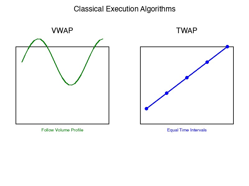

python

经典执行算法对比

现代执行算法：机器学习与强化学习#

1. 基于机器学习的成交量预测#

传统VWAP使用历史平均成交量作为预测，但现代算法使用机器学习模型预测未来成交量。

特征工程：

历史成交量模式（同时间段、同星期几）
市场状态（波动率、价差、订单簿深度）
事件驱动（财报、宏观数据发布）
另类数据（社交媒体情绪、新闻情感）

模型选择：

XGBoost/LightGBM：非线性关系 + 特征重要性
LSTM：捕捉时间序列依赖
Transformer：处理多资产、跨市场信息

Python示例（使用LightGBM）：

import lightgbm as lgb
import pandas as pd
import numpy as np

class MLVolumePredictor:
    def __init__(self):
        self.model = None
    
    def prepare_features(self, df):
        """构建特征"""
        features = pd.DataFrame()
        
        # 时间特征
        features['hour'] = df['timestamp'].dt.hour
        features['minute'] = df['timestamp'].dt.minute
        features['day_of_week'] = df['timestamp'].dt.dayofweek
        
        # 历史成交量
        for lag in [1, 5, 15, 30]:
            features[f'volume_lag_{lag}'] = df['volume'].shift(lag)
        
        # 波动率
        features['volatility'] = df['return'].rolling(20).std()
        
        # 价差
        features['spread'] = (df['ask'] - df['bid']) / df['mid']
        
        # 订单簿深度
        features['depth'] = df['bid_depth'] + df['ask_depth']
        
        return features.dropna()
    
    def train(self, df, target='volume'):
        """训练模型"""
        X = self.prepare_features(df)
        y = df.loc[X.index, target]
        
        # LightGBM训练
        train_data = lgb.Dataset(X, label=y)
        params = {
            'objective': 'regression',
            'metric': 'rmse',
            'learning_rate': 0.05,
            'num_leaves': 31,
        }
        
        self.model = lgb.train(params, train_data, num_boost_round=100)
    
    def predict(self, df):
        """预测成交量"""
        X = self.prepare_features(df)
        return self.model.predict(X)

python

2. 强化学习驱动的执行算法#

将执行问题形式化为马尔可夫决策过程（MDP）：

状态： $s_t$ = (剩余数量, 当前价格, 市场成交量, 时间)
动作： $a_t$ = 本时刻执行数量
奖励： $r_t$ = -（执行成本 + 市场冲击 + 时间风险）

DQN执行智能体：

import gym
import numpy as np
from stable_baselines3 import DQN

class ExecutionEnv(gym.Env):
    """执行环境"""
    def __init__(self, total_quantity, price_process, volume_process):
        super(ExecutionEnv, self).__init__()
        
        self.total_quantity = total_quantity
        self.price_process = price_process
        self.volume_process = volume_process
        
        # 动作空间：执行比例 [0, 1]
        self.action_space = gym.spaces.Box(low=0, high=1, shape=(1,), dtype=np.float32)
        
        # 状态空间：[剩余数量比例, 时间比例, 当前价格, 市场成交量]
        self.observation_space = gym.spaces.Box(
            low=0, high=np.inf, shape=(4,), dtype=np.float32
        )
        
        self.reset()
    
    def step(self, action):
        """执行一步"""
        # 计算执行数量
        execution_ratio = action[0]
        execute_quantity = self.remaining_quantity * execution_ratio
        
        # 计算市场冲击
        market_volume = self.volume_process[self.current_step]
        impact = 0.1 * (execute_quantity / market_volume) ** 0.5
        
        # 更新价格（市场冲击 + 随机波动）
        price_change = impact + np.random.normal(0, self.volatility)
        self.current_price *= (1 + price_change)
        
        # 计算执行成本
        execution_cost = execute_quantity * self.current_price * (1 + self.transaction_cost)
        
        # 更新状态
        self.remaining_quantity -= execute_quantity
        self.current_step += 1
        
        # 计算奖励（负的执行成本）
        reward = -execution_cost / self.total_quantity / self.initial_price
        
        # 是否完成
        done = (self.remaining_quantity <= 0) or (self.current_step >= len(self.price_process) - 1)
        
        # 构建新状态
        state = np.array([
            self.remaining_quantity / self.total_quantity,
            self.current_step / len(self.price_process),
            self.current_price,
            market_volume
        ], dtype=np.float32)
        
        return state, reward, done, {}
    
    def reset(self):
        """重置环境"""
        self.remaining_quantity = self.total_quantity
        self.current_step = 0
        self.current_price = self.price_process[0]
        self.initial_price = self.price_process[0]
        self.volatility = 0.01
        self.transaction_cost = 0.001
        
        return np.array([
            1.0,  # 剩余数量比例
            0.0,  # 时间比例
            self.current_price,
            0.0   # 市场成交量（需要初始化）
        ], dtype=np.float32)

# 训练DQN执行智能体
env = ExecutionEnv(total_quantity=100000, price_process=price_data, volume_process=volume_data)
model = DQN('MlpPolicy', env, verbose=1, learning_rate=1e-3)
model.learn(total_timesteps=50000)
model.save("dqn_execution_agent")

python

实盘挑战与解决方案#

1. 隐藏单与冰山单#

问题：大型订单会暴露交易意图，导致逆向选择。

解决方案：

隐藏单（Hidden Orders）：不显示在订单簿中
冰山单（Iceberg Orders）：只显示部分数量，定期刷新
暗池（Dark Pools）：在暗池中执行，不公开订单信息

Python示例（使用IB API）：

from ib_insync import *

# 连接Interactive Brokers
ib = IB()
ib.connect('127.0.0.1', 7497, clientId=1)

# 创建冰山单
contract = Stock('AAPL', 'SMART', 'USD')
order = Order(
    action='BUY',
    totalQuantity=100000,
    orderType='LMT',
    lmtPrice=150.0,
    hidden=True,  # 隐藏单
    displaySize=1000  # 冰山单：每次显示1000股
)

trade = ib.placeOrder(contract, order)
ib.sleep(1)
print(f"订单状态: {trade.orderStatus.status}")

python

2. 订单簿动态与微观结构#

问题：简单的市场冲击模型忽略订单簿动态。

解决方案：

订单簿深度学习：使用CNN/LSTM处理LOB数据
限价单vs市价单：根据订单簿深度动态选择
智能路由：在多个交易所之间分配订单

订单簿特征工程：

def extract_lob_features(lob_snapshot, levels=10):
    """提取订单簿特征"""
    features = []
    
    # 买卖价差
    spread = lob_snapshot['ask_price_0'] - lob_snapshot['bid_price_0']
    features.append(spread)
    
    # 加权中间价
    mid_price = (lob_snapshot['ask_price_0'] + lob_snapshot['bid_price_0']) / 2
    features.append(mid_price)
    
    # 订单簿不平衡
    for i in range(levels):
        bid_vol = lob_snapshot[f'bid_volume_{i}']
        ask_vol = lob_snapshot[f'ask_volume_{i}']
        imbalance = (bid_vol - ask_vol) / (bid_vol + ask_vol)
        features.append(imbalance)
    
    # 订单簿斜率（价格弹性）
    bid_slope = np.mean([lob_snapshot[f'bid_price_{i}'] - lob_snapshot[f'bid_price_{i+1}'] for i in range(levels-1)])
    ask_slope = np.mean([lob_snapshot[f'ask_price_{i+1}'] - lob_snapshot[f'ask_price_{i}'] for i in range(levels-1)])
    features.extend([bid_slope, ask_slope])
    
    return np.array(features)

python

3. 多资产执行与组合重构#

问题：需要同时执行多个资产的订单（如指数套利、组合重构）。

解决方案：

联合优化：考虑资产间的相关性
相对执行：保持组合权重不变
ETF创设/赎回：使用ETF作为执行工具

组合执行优化：

import cvxpy as cp

def optimize_portfolio_execution(orders, covariance_matrix, market_impact):
    """
    优化组合执行
    
    Parameters:
    -----------
    orders : dict
        {asset: quantity} 每个资产的执行数量
    covariance_matrix : np.ndarray
        资产收益率协方差矩阵
    market_impact : dict
        {asset: impact_coefficient} 市场冲击系数
    """
    n_assets = len(orders)
    assets = list(orders.keys())
    
    # 决策变量：每个资产的执行速率
    execution_rates = cp.Variable(n_assets)
    
    # 目标：最小化执行成本 + 组合风险
    execution_cost = cp.sum([market_impact[asset] * execution_rates[i]**2 for i, asset in enumerate(assets)])
    portfolio_variance = cp.quad_form(execution_rates, covariance_matrix)
    
    objective = cp.Minimize(execution_cost + 0.5 * portfolio_variance)
    
    # 约束：完成所有订单
    constraints = [cp.sum(execution_rates) == sum(orders.values())]
    
    # 求解
    problem = cp.Problem(objective, constraints)
    problem.solve()
    
    return {assets[i]: execution_rates.value[i] for i in range(n_assets)}

python

绩效评估与基准比较#

1. 执行质量指标#

VWAP偏差：执行均价与VWAP的差值
IS（Implementation Shortfall）：执行均价与决策时价格的差值
市场冲击：订单执行前后的价格变化
参与度：执行数量 / 市场成交量

2. 交易成本分析（TCA）#

def transaction_cost_analysis(orders, executions, benchmark_price='vwap'):
    """
    交易成本分析
    
    Parameters:
    -----------
    orders : list
        订单列表 [{timestamp, side, quantity, decision_price}]
    executions : list
        执行记录 [{timestamp, price, quantity}]
    benchmark_price : str
        基准价格（vwap, twap, decision）
    """
    results = []
    
    for order in orders:
        # 匹配执行记录
        order_executions = [e for e in executions if e['order_id'] == order['id']]
        
        # 计算加权平均执行价格
        total_quantity = sum([e['quantity'] for e in order_executions])
        weighted_price = sum([e['price'] * e['quantity'] for e in order_executions]) / total_quantity
        
        # 计算基准价格
        if benchmark_price == 'vwap':
            benchmark = calculate_vwap(order['start_time'], order['end_time'])
        elif benchmark_price == 'decision':
            benchmark = order['decision_price']
        
        # 计算执行成本
        if order['side'] == 'BUY':
            cost = weighted_price - benchmark
        else:
            cost = benchmark - weighted_price
        
        results.append({
            'order_id': order['id'],
            'side': order['side'],
            'quantity': total_quantity,
            'weighted_price': weighted_price,
            'benchmark': benchmark,
            'cost': cost,
            'cost_bps': cost / benchmark * 10000  # 基点
        })
    
    return pd.DataFrame(results)

python

总结#

最优执行算法是量化交易的最后一公里，直接决定了策略的实盘表现。

关键要点：

没有万能算法：VWAP适合被动跟踪，IS适合主动优化
机器学习赋能：成交量预测、市场冲击建模、强化学习执行
**实盘细节决定