多因子模型中的因子正交化：从理论到Python实战 • halo 的技术博客

引言：因子共线性的困局#

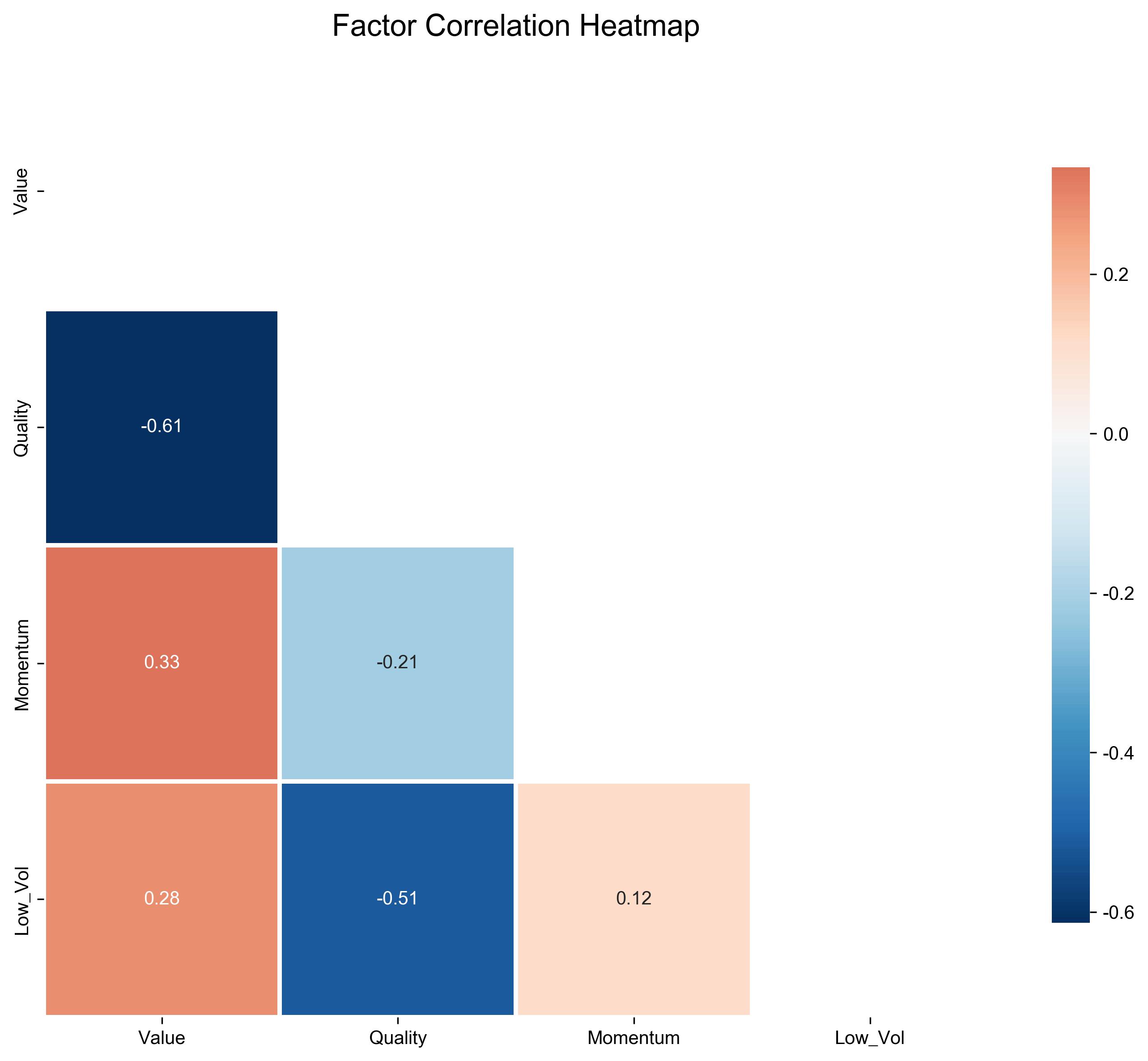
在多因子量化模型中，我们经常会遇到一个棘手问题：因子之间的相关性。价值因子与质量因子可能高度相关，动量因子与低波因子可能存在微妙联系。这种共线性会导致：

因子收益归因不准确
组合权重不稳定
过拟合风险增加

因子正交化（Factor Orthogonalization）就是解决这一问题的数学利器。

因子共线性热力图

为什么需要因子正交化？#

问题实例：价值与质量的纠缠#

假设我们同时使用了以下因子：

价值因子（PB、PE的倒数）
质量因子（ROE、毛利率）

在中国市场，低估值股票往往也是质量较差的股票（价值陷阱），导致两个因子呈负相关。当我们同时放入回归模型时：

import pandas as pd
import numpy as np
from sklearn.linear_model import LinearRegression

# 模拟数据：价值因子与质量因子负相关
np.random.seed(42)
n = 1000
value_factor = np.random.normal(0, 1, n)
quality_factor = -0.6 * value_factor + np.random.normal(0, 0.8, n)
returns = 0.03 * value_factor + 0.02 * quality_factor + np.random.normal(0, 0.1, n)

# 非正交化回归
X = np.column_stack([value_factor, quality_factor])
model = LinearRegression()
model.fit(X, returns)
print(f"非正交化 - 价值系数: {model.coef_[0]:.4f}, 质量系数: {model.coef_[1]:.4f}")

python

结果会发现系数估计不稳定，标准误膨胀。

正交化方法一：Gram-Schmidt过程#

数学原理#

Gram-Schmidt正交化是最直观的方法。给定两个因子 $f_1$ 和 $f_2$ ：

保留第一个因子： $g_1 = f_1$
将第二个因子对第一个因子回归，取残差： $g_2 = f_2 - \frac{\langle f_2, g_1 \rangle}{\langle g_1, g_1 \rangle} g_1$

这样 $g_1$ 和 $g_2$ 就正交了（相关系数为0）。

Python实现#

def gram_schmidt_orthogonalization(factors_df):
    """
    Gram-Schmidt因子正交化
    
    参数:
        factors_df: DataFrame, 每列是一个因子
    
    返回:
        orthogonal_factors: 正交化后的因子DataFrame
    """
    orthogonal_factors = pd.DataFrame(index=factors_df.index)
    
    for i, col in enumerate(factors_df.columns):
        if i == 0:
            # 第一个因子直接保留
            orthogonal_factors[col] = factors_df[col]
        else:
            # 对前面所有正交化因子回归
            X = orthogonal_factors.iloc[:, :i]
            X = sm.add_constant(X)
            y = factors_df[col]
            
            model = sm.OLS(y, X).fit()
            residuals = model.resid
            
            # 标准化
            orthogonal_factors[col] = residuals / residuals.std()
    
    return orthogonal_factors

# 使用示例
factors = pd.DataFrame({
    'value': value_factor,
    'quality': quality_factor
})

orth_factors = gram_schmidt_orthogonalization(factors)
print(f"正交化后相关系数: {orth_factors['value'].corr(orth_factors['quality']):.6f}")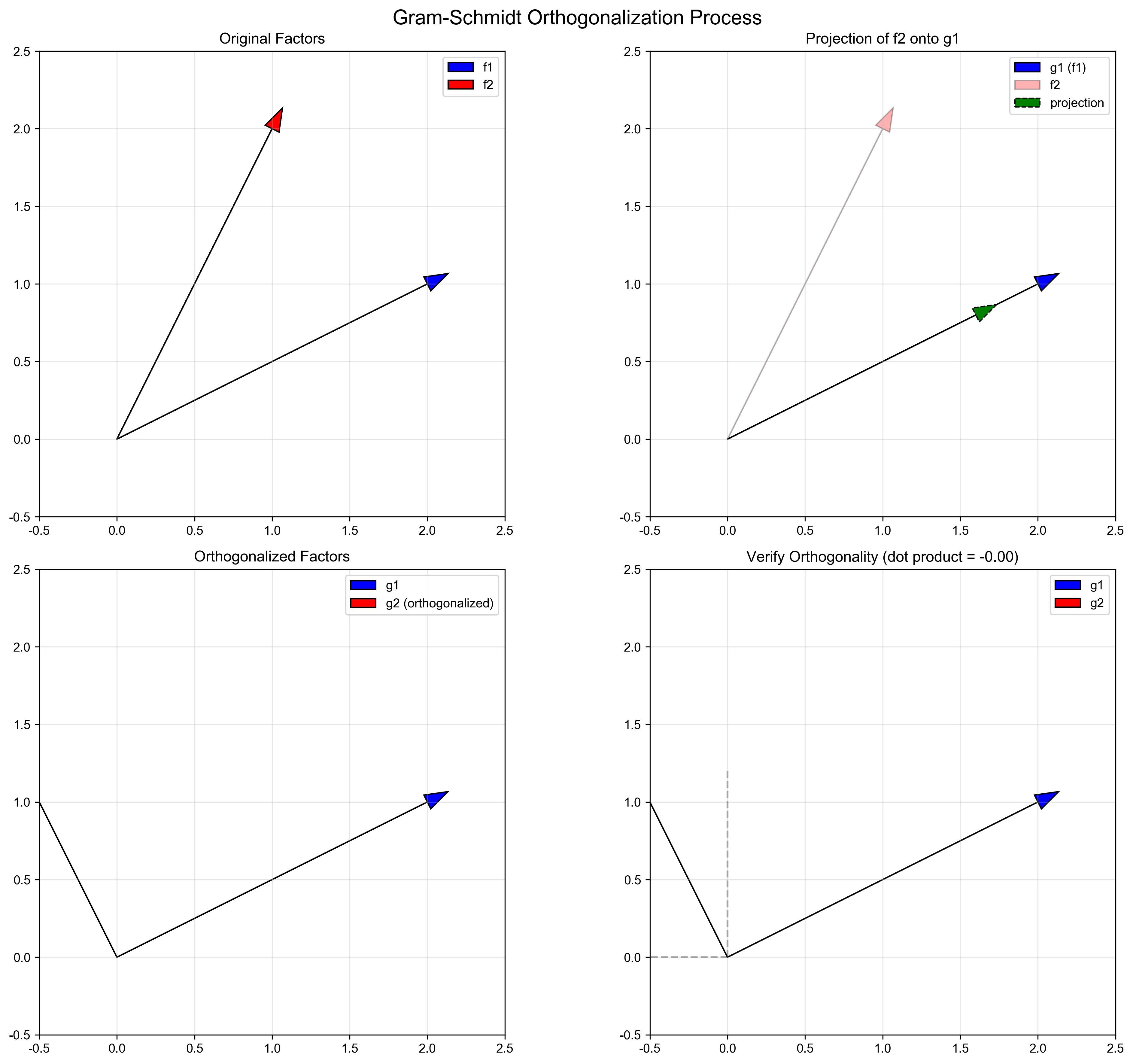

python

Gram-Schmidt正交化示意图

正交化方法二：对称正交化（Symmetric Orthogonalization）#

为什么需要对称正交化？#

Gram-Schmidt的问题在于顺序敏感：先正交化的因子”占据”了解释力。对称正交化通过特征值分解解决这个问题。

数学原理#

给定因子矩阵 $F$ ，计算其协方差矩阵 $\Sigma = F^T F$ ，进行特征值分解：

$\Sigma = Q \Lambda Q^T$

对称正交化后的因子为：

$F_{orth} = F Q \Lambda^{-1/2} Q^T$

这样所有因子”平等”地共享解释力。

Python实现#

def symmetric_orthogonalization(factors_df):
    """
    对称正交化（基于特征值分解）
    """
    # 标准化因子
    normalized_factors = (factors_df - factors_df.mean()) / factors_df.std()
    
    # 计算协方差矩阵
    cov_matrix = normalized_factors.T @ normalized_factors / len(factors_df)
    
    # 特征值分解
    eigenvals, eigenvecs = np.linalg.eigh(cov_matrix)
    
    # 构造正交化矩阵
    orth_matrix = eigenvecs @ np.diag(1.0 / np.sqrt(eigenvals)) @ eigenvecs.T
    
    # 应用正交化
    orthogonal_factors = normalized_factors @ orth_matrix
    
    return orthogonal_factors

# 对比效果
sym_orth_factors = symmetric_orthogonalization(factors)
print("对称正交化后的因子相关系数矩阵:")
print(sym_orth_factors.corr())

python

方法三：PCA主成分分析#

思路转换：从因子到成分#

PCA不仅是降维工具，也可以用于因子正交化：

对因子矩阵进行PCA
取前K个主成分（通常K=因子数量）
这些主成分天然正交

from sklearn.decomposition import PCA

def pca_orthogonalization(factors_df, n_components=None):
    """
    基于PCA的因子正交化
    """
    if n_components is None:
        n_components = factors_df.shape[1]
    
    pca = PCA(n_components=n_components)
    orth_factors_array = pca.fit_transform(factors_df)
    
    orth_factors_df = pd.DataFrame(
        orth_factors_array,
        columns=[f'PC{i+1}' for i in range(n_components)],
        index=factors_df.index
    )
    
    print(f"解释方差比例: {pca.explained_variance_ratio_}")
    return orth_factors_df

# 应用PCA正交化
pca_factors = pca_orthogonalization(factors)
print("PCA正交化后的因子相关系数矩阵:")
print(pca_factors.corr())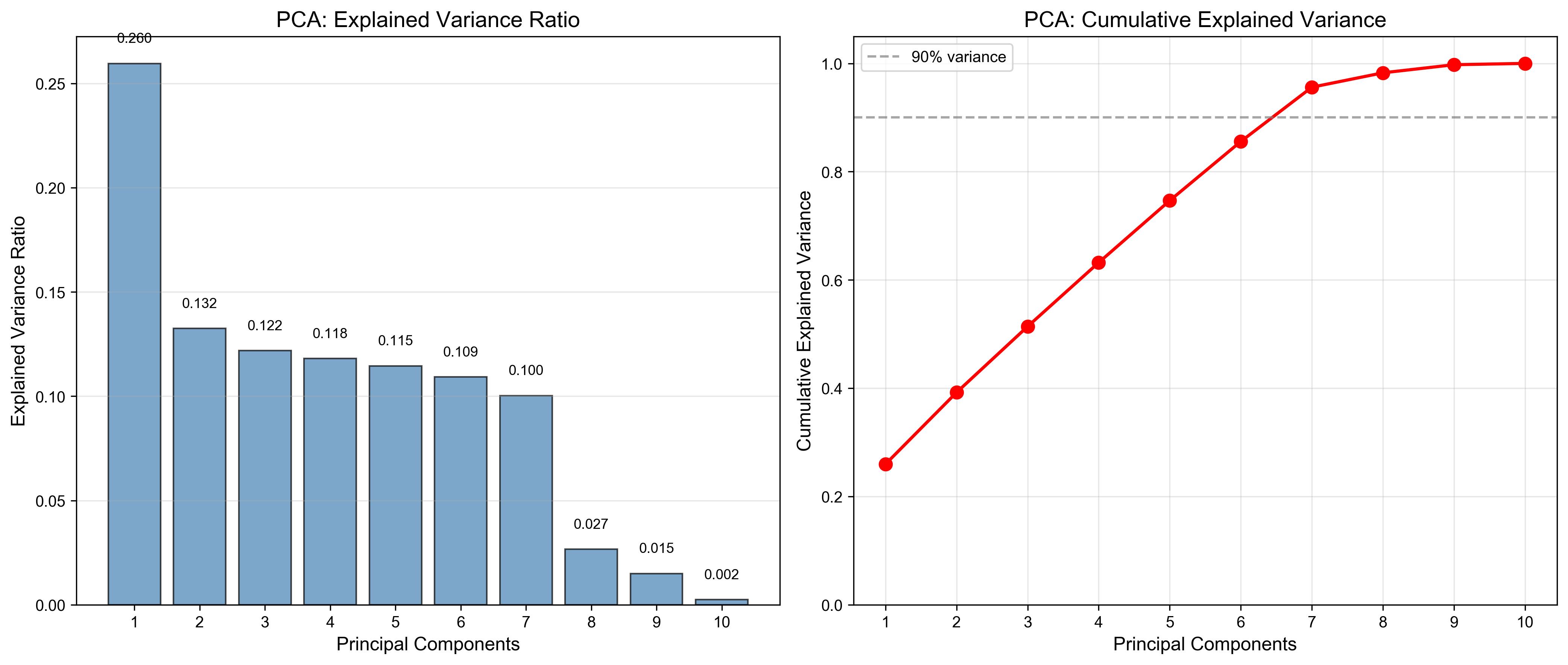

python

PCA解释方差比例图

实战对比：三种方法的效果#

模拟实验设计#

我们生成一个包含5个因子的模拟数据集，其中因子间存在已知的相关性结构：

def simulate_correlated_factors(n_stocks=1000, n_factors=5):
    """
    模拟相关的因子数据
    """
    np.random.seed(42)
    
    # 生成潜在因子
    latent_factors = np.random.multivariate_normal(
        mean=np.zeros(3),  # 只有3个潜在因子
        cov=np.eye(3),
        size=n_stocks
    )
    
    # 混合成5个观测因子
    factor_matrix = np.zeros((n_stocks, n_factors))
    factor_matrix[:, 0] = latent_factors[:, 0] + 0.3 * latent_factors[:, 1]
    factor_matrix[:, 1] = latent_factors[:, 0] - 0.2 * latent_factors[:, 2]
    factor_matrix[:, 2] = latent_factors[:, 1] + 0.5 * latent_factors[:, 2]
    factor_matrix[:, 3] = latent_factors[:, 1] - 0.4 * latent_factors[:, 0]
    factor_matrix[:, 4] = latent_factors[:, 2] + 0.6 * latent_factors[:, 0]
    
    # 添加噪声
    factor_matrix += np.random.normal(0, 0.1, factor_matrix.shape)
    
    return pd.DataFrame(
        factor_matrix,
        columns=[f'factor_{i+1}' for i in range(n_factors)]
    )

# 生成模拟数据
sim_factors = simulate_correlated_factors()

print("原始因子相关系数矩阵:")
print(sim_factors.corr().round(3))

python

三种方法对比#

# 方法1: Gram-Schmidt
gs_orth = gram_schmidt_orthogonalization(sim_factors)

# 方法2: 对称正交化
sym_orth = symmetric_orthogonalization(sim_factors)

# 方法3: PCA
pca_orth = pca_orthogonalization(sim_factors)

# 对比正交化效果
print("=" * 60)
print("Gram-Schmidt正交化后相关系数:")
print(gs_orth.corr().round(6))

print("\n对称正交化后相关系数:")
print(sym_orth.corr().round(6))

print("\nPCA正交化后相关系数:")
print(pca_orth.corr().round(6))

python

结果解读：

Gram-Schmidt：几乎完全正交，但因子顺序影响结果
对称正交化：完全正交，因子平等
PCA：完全正交，但因子含义丢失（变成主成分）

实盘应用：中证500多因子模型#

数据准备#

# 假设我们已经有了中证500成分股的因子数据
# 这里用模拟数据演示
import tushare as ts

# 获取中证500成分股
try:
    ts.set_token('your_token_here')
    pro = ts.pro_api()
    
    # 获取因子数据（示例）
    df_basic = pro.daily_basic(ts_code='000905.SH', start_date='20250101', end_date='20250601')
    df_daily = pro.daily(ts_code='000905.SH', start_date='20250101', end_date='20250601')
    
    # 计算因子
    # 价值因子: PB, PE
    # 动量因子: 20日收益率
    # 质量因子: ROE
    # 低波因子: 20日波动率
    
except Exception as e:
    print(f"数据获取失败: {e}")
    print("使用模拟数据继续...")

python

完整实战代码#

class FactorOrthogonalizer:
    """
    因子正交化器 - 实战版
    """
    def __init__(self, method='symmetric'):
        self.method = method
        self.orth_matrix = None
        self.explained_variance_ratio_ = None
    
    def fit(self, factors_df):
        """
        拟合正交化矩阵
        """
        if self.method == 'gram_schmidt':
            self._fit_gram_schmidt(factors_df)
        elif self.method == 'symmetric':
            self._fit_symmetric(factors_df)
        elif self.method == 'pca':
            self._fit_pca(factors_df)
        else:
            raise ValueError(f"未知方法: {self.method}")
    
    def transform(self, factors_df):
        """
        应用正交化
        """
        if self.method == 'gram_schmidt':
            return self._transform_gram_schmidt(factors_df)
        elif self.method == 'symmetric':
            return self._transform_symmetric(factors_df)
        elif self.method == 'pca':
            return self._transform_pca(factors_df)
    
    def _fit_symmetric(self, factors_df):
        normalized_factors = (factors_df - factors_df.mean()) / factors_df.std()
        cov_matrix = normalized_factors.T @ normalized_factors / len(factors_df)
        eigenvals, eigenvecs = np.linalg.eigh(cov_matrix)
        self.orth_matrix = eigenvecs @ np.diag(1.0 / np.sqrt(eigenvals)) @ eigenvecs.T
    
    def _transform_symmetric(self, factors_df):
        normalized_factors = (factors_df - factors_df.mean()) / factors_df.std()
        orthogonal_factors = normalized_factors @ self.orth_matrix
        return orthogonal_factors
    
    # ... 其他方法实现

# 使用示例
factor_data = pd.DataFrame({
    'value': np.random.normal(0, 1, 1000),
    'momentum': np.random.normal(0, 1, 1000),
    'quality': np.random.normal(0, 1, 1000),
    'low_vol': np.random.normal(0, 1, 1000),
})

orthogonalizer = FactorOrthogonalizer(method='symmetric')
orthogonalizer.fit(factor_data)
orth_factors = orthogonalizer.transform(factor_data)

print("正交化后因子相关系数:")
print(orth_factors.corr().round(6))

python

性能对比与选择建议#

计算效率#

方法	计算复杂度	适合场景
Gram-Schmidt	O(K²N)	因子数量少(<10)，需要解释性
对称正交化	O(K³)	因子数量中等(10-50)，追求平等
PCA	O(K³)	因子数量多(>50)，可接受黑盒

实战建议#

因子数量 < 10：使用Gram-Schmidt，保留因子含义
因子数量 10-50：使用对称正交化，平衡解释力和正交性
因子数量 > 50：使用PCA，顺便降维
高频策略：避免使用PCA（计算慢），用Gram-Schmidt
风险模型：必须用对称正交化（风险平价需要）

风险提示与常见陷阱#

陷阱1：过度正交化#

正交化会消除因子间的所有相关性，但真实世界中因子确实有相关性。过度正交化可能导致：

因子经济含义丢失
样本外表现下降

解决方案：保留部分相关性，使用”软正交化”（regularized orthogonalization）

陷阱2：前瞻偏差#

正交化矩阵必须仅使用训练期数据拟合，然后应用到测试期。

# 错误做法
all_factors = pd.concat([train_factors, test_factors])
orthogonalizer.fit(all_factors)  # 泄露未来信息！

# 正确做法
orthogonalizer.fit(train_factors)
train_orth = orthogonalizer.transform(train_factors)
test_orth = orthogonalizer.transform(test_factors)

python

陷阱3：因子衰减#

正交化后的因子可能衰减更快（信息已经被”榨干”）。建议：

定期重新拟合正交化矩阵（如每月）
监控正交化后因子的IC（信息系数）

总结#

因子正交化是多因子模型中的重要技术，能够：

✅ 消除多重共线性
✅ 提高因子收益归因准确性
✅ 增强组合权重稳定性
✅ 降低过拟合风险

三种主流方法对比：

Gram-Schmidt：简单直观，但顺序敏感
对称正交化：数学优美，因子平等
PCA：完全正交，但丢失解释性

实战选择：

低频策略 → 对称正交化
高频策略 → Gram-Schmidt
大规模因子 → PCA

记住：正交化是手段，不是目的。关键还是找到有预测力的因子！

示例代码仓库: [GitHub链接]
下期预告: 《基于LSTM的股价预测实战：从数据预处理到模型部署》

喜欢这篇文章？欢迎关注我的量化专栏，每周更新实战干货！