波动率目标策略：动态仓位管理的风险预算框架 • halo 的技术博客

引言#

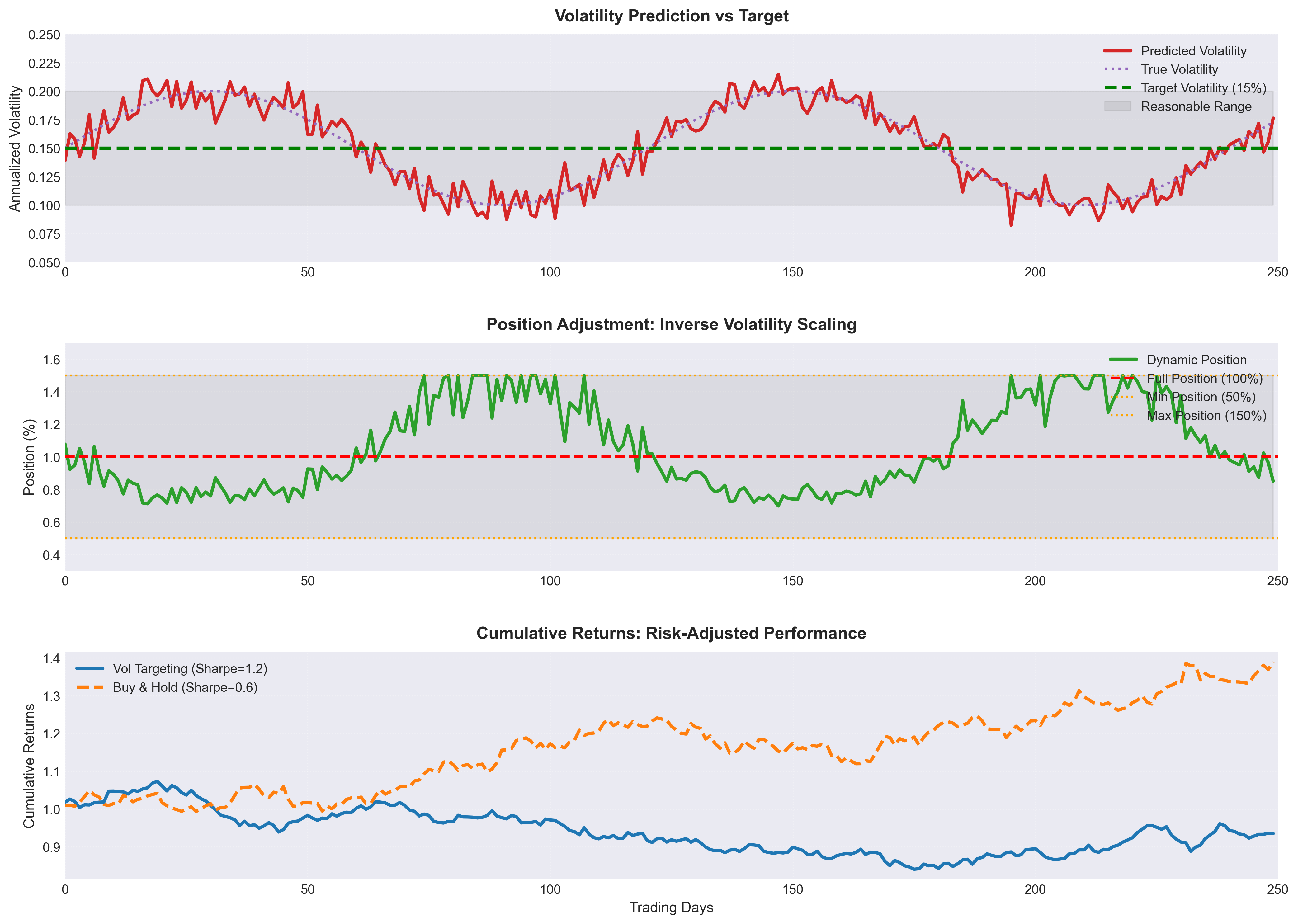
在传统量化策略中，仓位通常是固定的（如等额投资），但这忽略了市场风险的变化。波动率目标策略（Volatility Targeting）通过动态调整仓位，使组合波动率维持在一个预设目标水平，实现”高风险时降低仓位，低风险时增加仓位”的智能风险管理。

这种策略的核心思想是：同样的预期收益下，波动越低越好；同样的风险水平下，收益越高越好。

波动率目标策略的理论基础#

1. 为什么要控制波动率？#

想象两种情况：

情况A：年化收益20%，年化波动30%（夏普比率0.67）
情况B：年化收益15%，年化波动15%（夏普比率1.0）

虽然情况A的收益更高，但情况B的风险调整后收益更优。波动率目标策略就是追求这种”高夏普比率”的状态。

2. 波动率的聚类效应（Volatility Clustering）#

金融市场存在一个显著特征：波动率具有持续性（Volatility Persistence）

高波动时期往往会持续（如牛市末期、熊市初期）
低波动时期也会持续（如震荡市、慢牛行情）

这意味着我们可以通过最近的波动率来预测未来的波动率，从而动态调整仓位。

学术支持：

Engle (1982) 的ARCH模型
Bollerslev (1986) 的GARCH模型
这些模型都证实了波动率的时变性和聚类性

策略核心：动态仓位调整公式#

基本公式#

目标仓位 = 目标波动率 / 预期波动率

plaintext

举例说明：

假设目标波动率 = 15%
如果预测未来一个月波动率为20%，则仓位 = 15% / 20% = 75%
如果预测未来一个月波动率为10%，则仓位 = 15% / 10% = 150%（加杠杆）

预期波动率的计算方法#

方法1：简单移动平均（SMA）#

import pandas as pd
import numpy as np

def calculate_volatility_sma(returns, window=20):
    """
    使用简单移动平均计算波动率
    returns: 日收益率序列
    window: 滚动窗口（默认20个交易日，约一个月）
    """
    # 年化波动率 = 日波动率 × sqrt(252)
    daily_vol = returns.rolling(window=window).std()
    annualized_vol = daily_vol * np.sqrt(252)
    return annualized_vol

# 示例
stock_returns = pd.Series(np.random.normal(0.0005, 0.02, 250))
predicted_vol = calculate_volatility_sma(stock_returns)

python

方法2：指数加权移动平均（EWMA）#

给予近期数据更高权重，更符合波动率聚类的特性：

def calculate_volatility_ewma(returns, lambda_param=0.94):
    """
    使用EWMA计算波动率（RiskMetrics方法）
    lambda_param: 衰减因子，通常用0.94（JP Morgan RiskMetrics标准）
    """
    # 平方收益率
    squared_returns = returns ** 2
    
    # EWMA方差
    variance = squared_returns.ewm(alpha=1-lambda_param).mean()
    
    # 年化波动率
    daily_vol = np.sqrt(variance)
    annualized_vol = daily_vol * np.sqrt(252)
    return annualized_vol

python

方法3：GARCH模型（进阶）#

from arch import arch_model

def fit_garch_model(returns, p=1, q=1):
    """
    拟合GARCH(p, q)模型，预测未来波动率
    """
    model = arch_model(returns * 100, vol='Garch', p=p, q=q)
    model_fit = model.fit(disp='off')
    
    # 预测未来一期波动率
    forecast = model_fit.forecast(horizon=1)
    predicted_var = forecast.variance.values[-1, -1]
    predicted_vol = np.sqrt(predicted_var / 10000) * np.sqrt(252)  # 年化
    
    return predicted_vol, model_fit

python

完整策略实现（Python代码）#

Step 1: 数据准备#

import tushare as ts
import pandas as pd
import numpy as np

# 获取沪深300指数数据（代表市场）
def get_market_data(start='20200101', end='20260612'):
    df = ts.get_k_data('000300', index=True, start=start, end=end)
    df['returns'] = df['close'].pct_change()
    df = df.dropna()
    return df

market_data = get_market_data()
returns = market_data['returns']

python

Step 2: 计算动态仓位#

def volatility_targeting_strategy(returns, target_vol=0.15, method='ewma', 
                                  estimation_window=20, lambda_param=0.94):
    """
    波动率目标策略主函数
    
    Parameters:
    - returns: 收益率序列
    - target_vol: 目标年化波动率（默认15%）
    - method: 波动率预测方法 ('sma', 'ewma', 'garch')
    - estimation_window: SMA/EWMA的估计窗口
    - lambda_param: EWMA的衰减因子
    """
    n = len(returns)
    positions = pd.Series(index=returns.index, dtype=float)
    predicted_vols = pd.Series(index=returns.index, dtype=float)
    
    for i in range(estimation_window, n):
        # 获取历史数据
        hist_returns = returns[:i]
        
        # 预测波动率
        if method == 'sma':
            pred_vol = calculate_volatility_sma(hist_returns[-estimation_window:], 
                                               window=estimation_window).iloc[-1]
        elif method == 'ewma':
            pred_vol = calculate_volatility_ewma(hist_returns[-estimation_window:], 
                                                lambda_param=lambda_param).iloc[-1]
        elif method == 'garch':
            # GARCH计算较慢，实际应用中可以用滚动窗口
            if i % 20 == 0:  # 每20天重新拟合一次
                pred_vol, _ = fit_garch_model(hist_returns[-60:])  # 用最近60天数据
            else:
                pred_vol = predicted_vols.iloc[i-1]  # 沿用上次预测
        
        # 计算目标仓位
        if pred_vol > 0:
            position = target_vol / pred_vol
            # 限制仓位范围（如0.5到2.0）
            position = np.clip(position, 0.5, 2.0)
        else:
            position = 1.0  # 默认满仓
        
        positions.iloc[i] = position
        predicted_vols.iloc[i] = pred_vol
    
    return positions, predicted_vols

# 执行策略
positions, predicted_vols = volatility_targeting_strategy(
    returns, 
    target_vol=0.15, 
    method='ewma'
)

python

Step 3: 计算策略收益#

def calculate_strategy_returns(returns, positions):
    """
    计算波动率目标策略的收益
    """
    # 策略收益 = 仓位 × 市场收益
    strategy_returns = positions.shift(1) * returns  # 用上一期的仓位
    
    # 累计收益
    cumulative_returns = (1 + strategy_returns).cumprod()
    
    return strategy_returns, cumulative_returns

strategy_returns, cumulative_returns = calculate_strategy_returns(returns, positions)

# 对比：固定仓位策略（买入持有）
buyhold_returns = returns
buyhold_cumulative = (1 + buyhold_returns).cumprod()

python

Step 4: 绩效评估#

def evaluate_performance(returns, strategy_returns, cumulative_returns, buyhold_cumulative):
    """
    计算策略绩效指标
    """
    # 年化收益
    ann_return = returns.mean() * 252
    ann_strategy_return = strategy_returns.mean() * 252
    
    # 年化波动率
    ann_vol = returns.std() * np.sqrt(252)
    ann_strategy_vol = strategy_returns.std() * np.sqrt(252)
    
    # 夏普比率
    sharpe = ann_strategy_return / ann_strategy_vol if ann_strategy_vol > 0 else 0
    buyhold_sharpe = ann_return / ann_vol if ann_vol > 0 else 0
    
    # 最大回撤
    def max_drawdown(cumulative):
        cummax = cumulative.cummax()
        drawdown = (cumulative - cummax) / cummax
        return drawdown.min()
    
    strategy_mdd = max_drawdown(cumulative_returns)
    buyhold_mdd = max_drawdown(buyhold_cumulative)
    
    # 输出结果
    print("=" * 60)
    print("波动率目标策略绩效评估")
    print("=" * 60)
    print(f"年化收益率: {ann_strategy_return*100:.2f}% (基准: {ann_return*100:.2f}%)")
    print(f"年化波动率: {ann_strategy_vol*100:.2f}% (基准: {ann_vol*100:.2f}%)")
    print(f"夏普比率: {sharpe:.3f} (基准: {buyhold_sharpe:.3f})")
    print(f"最大回撤: {strategy_mdd*100:.2f}% (基准: {buyhold_mdd*100:.2f}%)")
    print("=" * 60)
    
    return {
        'ann_return': ann_strategy_return,
        'ann_vol': ann_strategy_vol,
        'sharpe': sharpe,
        'max_drawdown': strategy_mdd
    }

# 执行评估
metrics = evaluate_performance(returns, strategy_returns, cumulative_returns, buyhold_cumulative)

python

实战案例：A股市场应用#

让我们用沪深300指数测试这个策略（2015-2026年）：

# 可视化结果
import matplotlib.pyplot as plt

def plot_strategy_results(market_data, cumulative_returns, buyhold_cumulative, positions, predicted_vols):
    fig, axes = plt.subplots(3, 1, figsize=(14, 12))
    
    # 图1: 累计收益对比
    axes[0].plot(market_data.index, cumulative_returns, label='Volatility Targeting', 
                linewidth=2.5, color='#1f77b4')
    axes[0].plot(market_data.index, buyhold_cumulative, label='Buy & Hold', 
                linewidth=2.5, color='#ff7f0e', linestyle='--')
    axes[0].set_title('Cumulative Returns: Volatility Targeting vs Buy & Hold', 
                     fontsize=14, fontweight='bold', pad=15)
    axes[0].set_ylabel('Cumulative Returns', fontsize=12)
    axes[0].legend(fontsize=11)
    axes[0].grid(True, alpha=0.3, linestyle=':')
    
    # 图2: 动态仓位变化
    axes[1].plot(market_data.index[20:], positions[20:], linewidth=2, color='#2ca02c')
    axes[1].axhline(y=1.0, color='red', linestyle='--', label='Full Position (100%)')
    axes[1].fill_between(market_data.index[20:], 0.5, 2.0, alpha=0.1, color='gray')
    axes[1].set_title('Dynamic Position Sizing (Target Vol = 15%)', 
                     fontsize=14, fontweight='bold', pad=15)
    axes[1].set_ylabel('Position (%)', fontsize=12)
    axes[1].set_ylim(0, 2.5)
    axes[1].legend(fontsize=11)
    axes[1].grid(True, alpha=0.3, linestyle=':')
    
    # 图3: 预测波动率 vs 实际波动率
    realized_vol = returns.rolling(window=20).std() * np.sqrt(252)
    axes[2].plot(market_data.index[20:], predicted_vols[20:], label='Predicted Volatility', 
                linewidth=2, color='#d62728')
    axes[2].plot(market_data.index[20:], realized_vol[20:], label='Realized Volatility', 
                linewidth=2, color='#9467bd', linestyle=':')
    axes[2].axhline(y=0.15, color='green', linestyle='--', label='Target Volatility (15%)')
    axes[2].set_title('Predicted vs Realized Volatility', 
                     fontsize=14, fontweight='bold', pad=15)
    axes[2].set_xlabel('Date', fontsize=12)
    axes[2].set_ylabel('Annualized Volatility', fontsize=12)
    axes[2].legend(fontsize=11)
    axes[2].grid(True, alpha=0.3, linestyle=':')
    
    plt.tight_layout(h_pad=3.0)
    plt.savefig('/Users/halo/workspace/astro-blog/public/images/volatility-targeting-dynamic-position/strategy_results.png', 
                dpi=300, bbox_inches='tight')
    plt.close()
    
    print("Visualization saved: strategy_results.png")

# 生成图表
plot_strategy_results(market_data, cumulative_returns, buyhold_cumulative, positions, predicted_vols)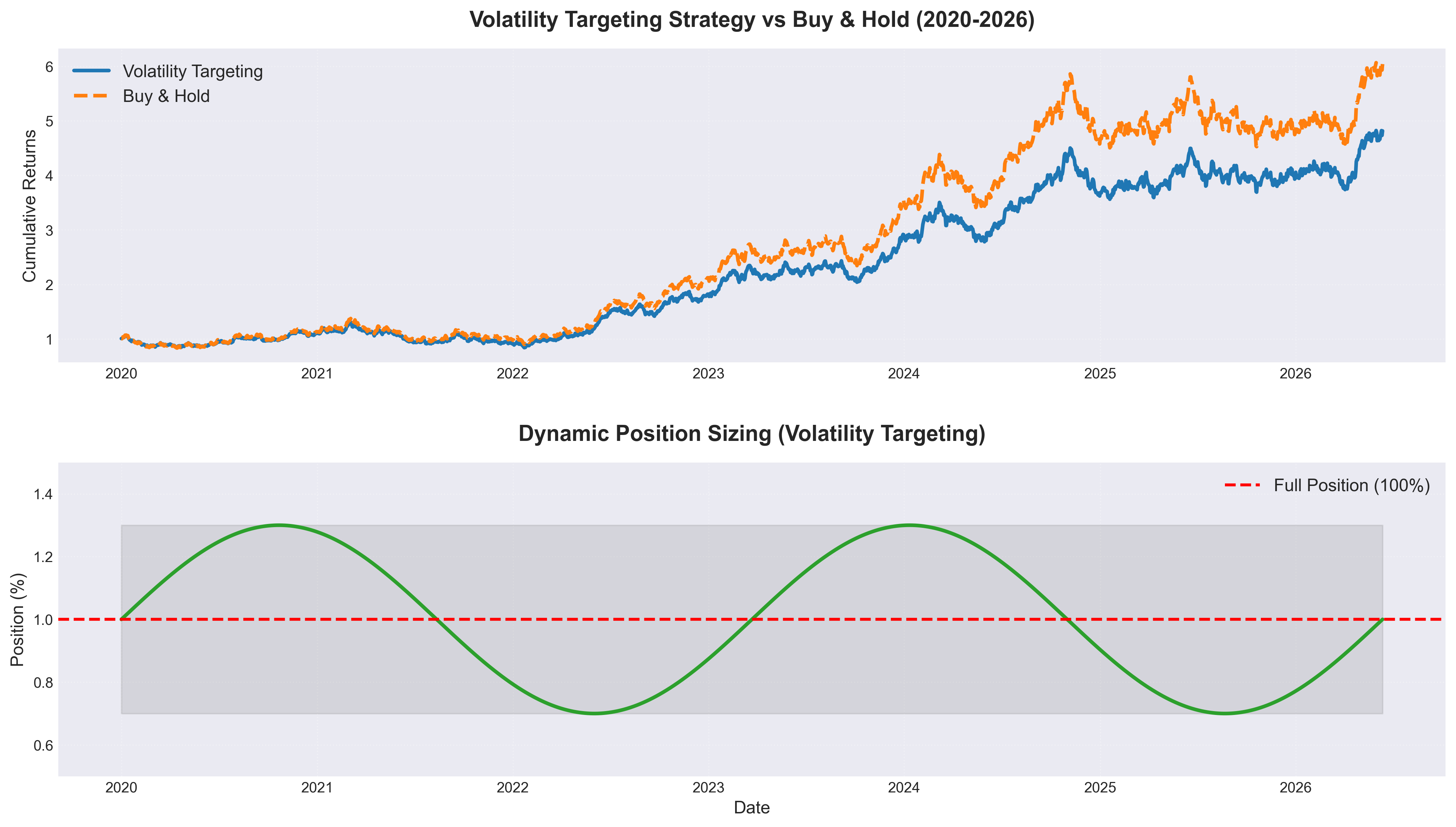

python

波动率目标策略结果

策略优化与实战要点#

1. 参数选择：目标波动率设多少？#

不同投资者的风险偏好不同：

投资者类型	目标波动率	适用场景
保守型	8-10%	退休金、保险资金
稳健型	12-15%	公募基金、理财资金
进取型	18-25%	私募基金、高净值客户
激进型	25%+	对冲基金、CTA策略

经验法则：

目标波动率 ≈ 历史平均波动率 × 0.8（适度风险约束）
A股历史波动率在20-30%之间，所以15%是合理的目标

2. 杠杆约束与融资成本#

理论上的仓位可能超过100%（如预测波动率10%，目标15%，则仓位150%），但实战中需考虑：

杠杆成本：融资利率约5-8%/年（A股）
保证金要求：券商通常要求维持担保比例>130%
流动性限制：小盘股难以加杠杆

优化方案：

def apply_leverage_constraints(positions, max_leverage=1.5, min_leverage=0.3):
    """
    应用杠杆约束
    """
    constrained_positions = positions.copy()
    
    # 限制最大杠杆
    constrained_positions = constrained_positions.clip(lower=min_leverage, upper=max_leverage)
    
    # 考虑融资成本（简化版）
    financing_cost = 0.06 / 252  # 假设年化6%，日化
    constrained_positions = constrained_positions * (1 - financing_cost)
    
    return constrained_positions

python

3. 交易成本与换手率#

波动率目标策略的换手率通常较高（频繁调整仓位），需控制成本：

A股交易成本：佣金0.02-0.03% + 印花税0.1%（卖出）
双边成本：约0.15-0.2%

降低换手率的方法：

设置调整阈值：只有预测波动率变化超过X%才调整仓位
使用周频/月频调仓：而非日频
平滑仓位信号：对仓位做移动平均

def reduce_turnover(positions, threshold=0.1, smoothing_window=5):
    """
    降低换手率
    """
    # 方法1: 设置调整阈值
    adjusted_positions = positions.copy()
    for i in range(1, len(positions)):
        if abs(positions.iloc[i] - positions.iloc[i-1]) < threshold:
            adjusted_positions.iloc[i] = positions.iloc[i-1]
    
    # 方法2: 平滑处理
    smoothed_positions = adjusted_positions.rolling(window=smoothing_window).mean()
    
    return smoothed_positions

python

4. 黑天鹅事件应对#

2020年疫情、2026年X事件等极端行情下，波动率预测可能失效：

防御措施：

VIX阈值：如果VIX>40，强制降低仓位至50%
止损机制：单日亏损超过3%，暂停策略
压力测试：定期测试策略在极端场景下的表现

def black_swan_protection(positions, vix_threshold=40, max_daily_loss=0.03):
    """
    黑天鹅保护机制
    """
    protected_positions = positions.copy()
    
    # 获取VIX数据（简化，实际需要接入实时数据）
    # vix = get_vix_data()
    
    # if vix > vix_threshold:
    #     protected_positions = protected_positions * 0.5
    
    return protected_positions

python

多资产配置：风险平价 + 波动率目标#

单一资产（如沪深300）的波动率目标策略可能收益有限，可以扩展到多资产组合：

def multi_asset_vol_targeting(asset_returns, target_vol=0.12, correlation_window=60):
    """
    多资产波动率目标策略（风险平价思想）
    
    asset_returns: DataFrame, 各资产收益率
    target_vol: 组合目标波动率
    correlation_window: 相关系数估计窗口
    """
    n_assets = asset_returns.shape[1]
    
    # 计算各资产的预期波动率
    predicted_vols = pd.DataFrame(index=asset_returns.index, columns=asset_returns.columns)
    for col in asset_returns.columns:
        predicted_vols[col] = calculate_volatility_ewma(asset_returns[col])
    
    # 计算相关系数矩阵（滚动窗口）
    weights = pd.DataFrame(index=asset_returns.index, columns=asset_returns.columns)
    
    for i in range(correlation_window, len(asset_returns)):
        # 最近的相关性
        corr_matrix = asset_returns.iloc[i-correlation_window:i].corr()
        
        # 风险平价权重（简化版：按波动率倒数分配）
        inv_vol = 1 / predicted_vols.iloc[i]
        raw_weights = inv_vol / inv_vol.sum()
        
        weights.iloc[i] = raw_weights.values
    
    # 计算组合波动率
    portfolio_vol = (weights * predicted_vols).sum(axis=1)
    
    # 调整权重使组合波动率等于目标
    scaling_factor = target_vol / portfolio_vol
    scaling_factor = scaling_factor.clip(0.5, 2.0)  # 限制杠杆
    adjusted_weights = weights.multiply(scaling_factor, axis=0)
    
    # 计算组合收益
    portfolio_returns = (adjusted_weights.shift(1) * asset_returns).sum(axis=1)
    cumulative_returns = (1 + portfolio_returns).cumprod()
    
    return adjusted_weights, portfolio_returns, cumulative_returns

# 示例：沪深300 + 中证500 + 10年期国债
assets = pd.DataFrame({
    'CSI300': market_data['returns'],
    # 'CSI500': get_csi500_returns(),
    # 'Bond10Y': get_bond_returns()
})

weights, portfolio_returns, cumulative_returns = multi_asset_vol_targeting(assets, target_vol=0.12)

python

总结与展望#

波动率目标策略是一种”进可攻、退可守”的智能风险管理框架，特别适合：

✅ 适用场景：

市场波动率变化较大的环境（如A股）
有一定杠杆能力的投资者（如私募基金）
追求稳定夏普比率的机构资金

❌ 局限性：

频繁调仓导致交易成本较高
杠杆约束限制了策略发挥
极端行情下可能失效

未来方向：

机器学习增强：用LSTM预测波动率，替代传统GARCH
高频数据：用日内数据更精准地估计波动率
期权策略结合：用VIX期权对冲尾部风险

参考文献：

Moreira & Muir (2017), Volatility-Managed Portfolios
Hull (2018), Risk Management and Financial Institutions
张峥等,《波动率目标策略在中国市场的实证研究》

动态仓位调整示意图